Stellar FabricThermal states and the source–geometry test
A positive energy gate, a negative local null stress, and a closer static match—tested within one declared model.
By Stan Schneider
Published
Thermal states · source and geometry
Conceptual geometry · not a computed solution
FROM PREPARATION TO A THERMAL BRANCH
The state and the geometry have to agree.
We compared the stress generated by a quantum field with the stress a proposed geometry would require. The calculations move from the effects of a finite pulse to the vacuum and thermal states of an interacting model, testing both the energy balance and the static field equations.
The most recent step is a nonconstant thermal approximation with a much smaller static-tensor residual. On one inherited fixed geometry, proper energy also becomes positive before the local negative null sign is lost. These are separate calculations; a compatible energy sign does not by itself solve the geometry.
SCIENTIFIC STATUS · OCTOBER 16
The latest thermal branch is an approximate stationary result on a closed periodic cell at a finite prescription. Physical source admission, exterior completion, full joint stability, preparation and loading remain unresolved.
See the earlier overview for the finite bare-field calculation. It uses different quantities and assumptions from the renormalized model.
SEVEN FINDINGS · EQUATIONS & CHECKS
Show the source. Then test the match.
Each entry links the established framework to the calculation made in this project. The tables show the checks and their results. Exact identities and numerical approximations are distinguished throughout.
Notation is local to each entry. Quantities use the stated normalized model units, with c=ℏ=1. Temperature numbers are not kelvin. The leading-order large-N scalar approximation, fixed-background tests and finite-regulator geometry search are identified separately. Long equations scroll within their own blocks on small screens.
The long-time average after one smooth pulse is nonnegative.
Conditional analytical result · fixed free field
A finite pulse can create intervals of negative reference-subtracted null stress. In the stated gapped free-field problem, the infinite-time average after the pulse is nevertheless nonnegative. This restricts the idea of preparing a permanent negative support once and then switching the drive off.
Established starting point
The Hadamard in/out-state construction for asymptotically static Klein–Gordon fields is established by Gérard and Wrochna. We use its hypotheses for the smooth companion problem; the theorem itself is not a project invention. [1]
What we derived or checked
We derived the postpulse null-increment average, retained exactly degenerate occupation coherences, and checked the finite Gaussian decomposition separately from the continuum argument.
(01.1)
(01.2)
𝒩± is a positively smeared radial-null observable; Δ is its difference from the original vacuum. The pulse returns exactly to the original positive, gapped quadratic Hamiltonian. T is pulse completion time, S the averaging duration, and Cλ the degenerate-frequency block of Cmn=⟨a†m an⟩, a positive semidefinite occupation covariance. Bλ is the associated weighted Gram matrix; superscript T denotes transpose. These symbols are local to this result.
Tests & outcome
Checks for result 01: What a completed pulse leaves behind
Check
Result
Finite covariance identity
All 62 algebra checks passed; maximum decomposition error 4.72×10⁻¹⁶. A deliberately wrong transpose gives an error of about 0.0707.
Continuum scope
For the C∞ companion, the argument uses a smooth covariance difference on compact space. The sin⁴ switching pulse is only C³ and keeps the finite-regulator claim.
Derivation & model scope
After the drive ends, expand the positive null square into occupation and anomalous pair terms.
A positive gap prevents the pair sum from having zero frequency. Its Cesàro mean vanishes; degenerate occupation coherences remain in positive Gram blocks.
Use the smooth-state hypotheses to justify the continuum averaging step; a finite numerical trace is a separate control.
The geometry and the postpulse quadratic Hamiltonian are fixed. This is a statement about a time average, not the duration of every negative interval. Some long driven protocols fail their direct energy-balance test; those runs are not used as a continuum proof.
The change from the original vacuum and the absolute source are different quantities.
What remains unresolvedContinuing drives, interactions, dissipation and geometry feedback need their own analysis. This result does not determine the absolute vacuum baseline or exclude all wormholes.
02
Source accounting
A conserved relative source includes the response of the medium.
We compared one periodic cell with repeated copies of precisely the same local geometry and action. Varying that common relative functional gives the scalar density, both pressures and the mean-field forces. The induced classical response then closes the retained first-loop conservation balance.
Established starting point
Topological Casimir subtraction is established in compactification calculations. Conservation from a common stress/mean-field action is established quantum-field methodology. Neither method identifies a complete supporting source by itself. [2] [3]
What we derived or checked
We computed the full relative scalar tensor and its induced η/Maxwell response on the chosen nonuniform cell, then compared independent spectral and differential-equation routes.
(02.1)
(02.2)
q counts identical cells, not a stretched copy. φ is the quantum scalar, η the classical normalization field and B the Maxwell sector in this calculation. ΔT is a relative tensor, not an absolute vacuum tensor. The induced fields are solved with the same boundary conditions and first-loop ordering.
Tests & outcome
Checks for result 02: Include the medium response
Check
Result
Dressed conservation · 2048 spatial points
Maximum Ward residual 1.51×10⁻¹⁰, compared with 1.04×10⁻⁷ for the scalar contribution alone. The detector null contrast is −0.02343026.
Independent representation
Matched angular/frequency limits give a tested extrapolated-observable difference of about 4.03×10⁻¹¹. It is an empirical comparison, without a rigorous tail enclosure.
Size of the retained contrast
The detector contrast is about 8.44×10⁻⁶ of the selected geometric deficit. The unknown absolute cover source is not set to zero.
Derivation & model scope
Repeat every local variation in every cover cell before dividing by q; purely local finite action terms then cancel in the contrast.
Vary the same relative functional with respect to the metric and retained mean fields.
Add the induced classical η and Maxwell response at the same loop order, and check the resulting Ward balance.
The cover is not empty Minkowski space. Other quantum sectors and a complete self-consistent mean solution are absent. An additional conditional comparison shows that the strongest topology-induced χ softening is radial; it does not prove joint matter–geometry stability.
The source and the response of the medium are varied together, with the same boundary conditions.
What remains unresolvedThis partial relative source does not close the absolute Einstein source or supply the missing geometric stress.
03
Renormalized vacuum
A specified renormalized scalar sector has a positive gap and negative radial-null stress.
Declared leading-order large-N model · analytic sign and numerical checks
The new uniform-product calculation goes beyond a negative reference increment. One covariantly subtracted functional defines the interacting scalar saddle and its absolute sector tensor. In its untwisted vacuum, the radial-null component is negative while the self-consistent frequency gap is positive.
Established starting point
Heat-kernel subtraction and consistent curved-space effective-action mean equations are established tools. The cited Hartree examples use different backgrounds and approximations; their solutions are not imported into this calculation. [4] [5]
What we derived or checked
We solved the chosen leading-order large-N product model with its declared finite inputs, evaluated the source and response from one functional, and tested the massless-input and geometric-parameter cases.
(03.1)
(03.2)
u is the self-consistent mass squared, ρR the renormalized field variance, h the scalar–χ coupling and gR the positive effective quartic coupling. Wwind is the winding part of the renormalized scalar functional WR, not the full stationary density Von=WR−gRρR²/4. Its L derivative holds the independent u and means fixed before stationarity. L is circle length, and Tkk=ℰ+pr uses the metric-normalized radial null direction. The approximation retains the leading order for many identical scalar species; quoted densities are per species in model units.
Tests & outcome
Checks for result 03: An absolute sector component is now defined
Check
Result
Reference input mR²=0.05
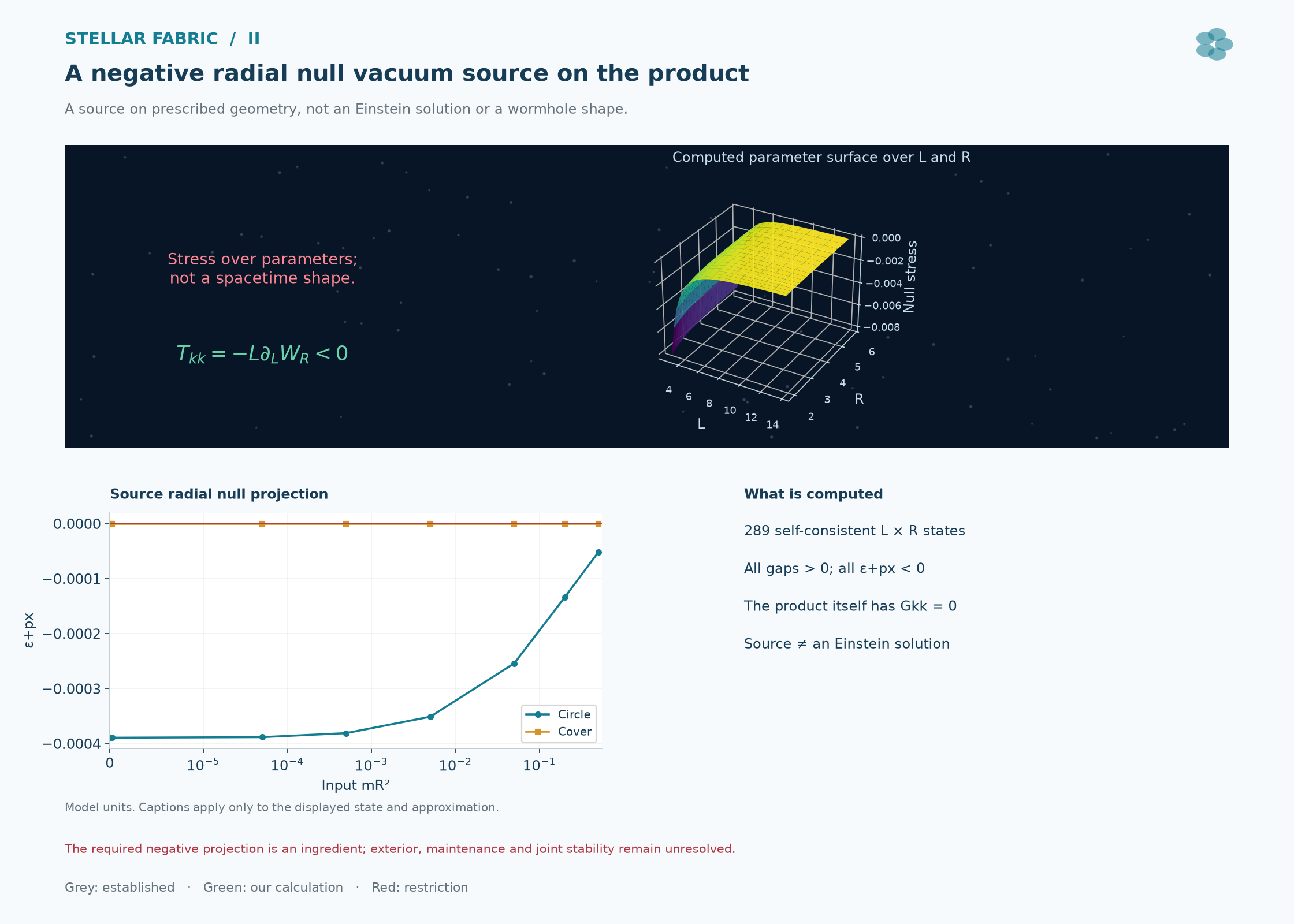
u=0.05000168885; √u=0.2236105741; Tkk=−2.5430370187×10⁻⁴. The gap-equation residual is about 1.90×10⁻¹⁵.
Zero input mass
At mR²=0, the interacting saddle retains u=9.284699789×10⁻⁵ and √u≈0.009635715; Tkk≈−3.894717628×10⁻⁴.
Parameter and response controls
All 289 tested length/radius states have a positive gap and negative sector Tkk. The separate bounded uniform vacuum response test does not establish the full spectrum.
Derivation & model scope
Fix the local subtraction prescription and the finite action inputs before solving the stationary gap equation.
Differentiate that same stationary functional for the pressures. In the uniform vacuum the radial-null combination retains the winding derivative.
Compare the resulting source with the assigned geometry: the constant product has Gkk=0, while this sector has Tkk<0. It therefore does not solve that Einstein equation by itself.
The result concerns the leading-order large-N scalar sector on assigned S¹×S², with explicit but unmeasured finite inputs. Subleading χ, η and gauge loops and joint metric dynamics are not included. The earlier finite bare-null positivity result remains valid in its own scope; it is not a statement about this renormalized tensor.
This renormalized model and the finite bare-field calculation use different assumptions.
What remains unresolvedA negative absolute sector component is now defined, but a physically normalized complete source and a self-consistent wormhole remain open.
A negative sector source, on an assigned productThe renormalized calculation produces a negative radial-null source over the displayed self-consistent parameter family. The upper surface plots stress over L and R; it is not a spacetime shape. The lower panel compares the compact circle and cover. The prescribed product geometry is not a joint Einstein solution.Open full-size research figure ↗
04
Thermal equilibrium
Thermal equilibrium is imposed on the original four-dimensional operator.
Specified Gaussian KMS source · finite regulator
With a spatially varying clock rate, adding thermal occupation numbers to an old constant-lapse spectrum is insufficient. We recomputed the selected Gaussian equilibrium state, its mean fields and its three static source components using one four-dimensional functional.
Established starting point
KMS equilibrium, the Tolman–Ehrenfest temperature relation and Euclidean thermal continuation are established. The project applies them to the chosen interacting mean-field approximation; the temperature law is not a new discovery. [6] [7] [4]
What we derived or checked
We retained the original lapse-dependent operator in the Matsubara sum and used the same regulator and local subtraction for each metric and mean-field variation.
(04.1)
(04.2)
(04.3)
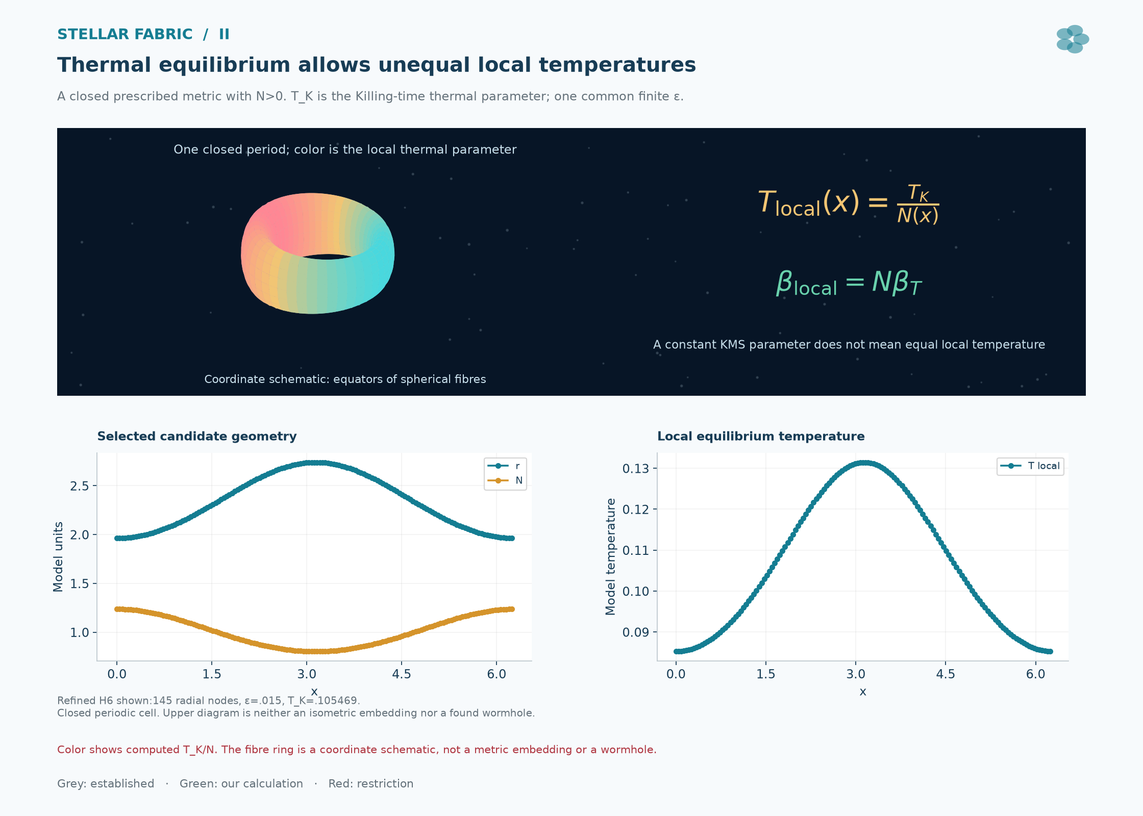
ds²=−N(x)²dt²+B(x)²dx²+r(x)²dΩ² on a closed periodic spatial cell, with N,B,r>0. Tg is Killing temperature; Tlocal is local equilibrium temperature. νn is a Matsubara frequency, ℓ an angular index, E1 the exponential integral and ε the proper-time cutoff. N here is lapse, not species count or spatial resolution.
Tests & outcome
Checks for result 04: Change the state within the same action
Check
Result
Thermodynamic normalization
An independent centered difference of re-solved F(Tg±h), with h=10⁻⁴, gives relative error 1.13×10⁻⁶ in the temperature-normalization test.
Repeat calculation from a fresh start
Three selected states were recomputed separately with the same numerical algorithm; all 231 comparisons passed. The maximum difference among the selected mean/source arrays is about 4.5×10⁻¹².
Derivation & model scope
Set the global Euclidean period and preserve the lapse multiplication on both sides of the frequency operator.
Solve the retained scalar variance and χ mean together by stationarity of Fψ+Emean.
Vary the same finite prescription for the source. The displayed operator relation is a congruence, not a similarity, so its eigenvalues cannot be shifted as if N were constant.
The raw free-energy formula is completed by the same declared local subtraction and classical mean energy used throughout the calculation. Entropy is defined from (EK−F)/Tg; that identity alone is not an independent entropy test. The centered-difference check is separate.
The temperature is changed within the same four-dimensional source model.
What remains unresolvedA finite equilibrium state is specified mathematically; an actual thermal bath, preparation protocol and finite reservoir have not been supplied.
05
Energy balance
Heating removes one cold obstruction before the local negative stress disappears.
Computed thermal window · one fixed inherited geometry
On the geometry inherited from the earlier cold joint attempt, thermal excitation makes integrated proper energy positive while the source at the sampled minimum radius still has negative Tkk. These necessary signs coexist over a bounded temperature interval in this family.
Established starting point
In a static gravitational field, free energy, Killing energy and proper-slice energy are different quantities. Their thermodynamic and metric definitions are established; the project tests their simultaneous compatibility in one specified source family. [8] [7] [9]
What we derived or checked
We re-solved the means across temperature on the same inherited geometry and kept its proper-energy crossing separate from the local null-sign crossing and the later geometry search.
(05.1)
(05.2)
ℰ is the local energy density and dV₃=4πr²dl. S is entropy, rl=dr/dl and κ the positive compatibility coefficient in G=κT. The second identity is the integrated static Gtt requirement for the declared closed spherical cell with Λ=0. It is a necessary condition, not the complete Einstein system.
Tests & outcome
Checks for result 05: Positive proper energy and a negative local sign
Check
Result
Same fixed geometry · ε=0.12, 49 points
At Tg=0: Eproper=−0.0156381811. At Tg=0.1: Eproper=+0.0379961598, while minimum-radius Tkk=−1.2741873×10⁻⁵.
Two empirical threshold brackets · ε=0.12, 49 points
In this inherited-geometry family, the proper-energy crossing is bracketed by Tg∈[0.07345703125, 0.073515625]; loss of the minimum-radius negative sign is bracketed by [0.10888671875, 0.108984375]. These finite-resolution brackets are not interval certificates or an exhaustive search. Temperatures use model units, not kelvin.
Derivation & model scope
Keep the inherited cold geometry fixed while changing only the equilibrium state and re-solving its means.
Compute both energy integrals with their correct lapse weights; the uniform-lapse variation tests EK, whereas the proper-volume Einstein gate tests Eproper.
Track the local null sign at the same minimum-radius sample. The distinct crossings define a compatibility window, not a solved metric.
This thermal test keeps the geometry fixed; it does not solve the Einstein equations. The order of the two sign changes depends on the chosen geometry. A separate cold calculation failed a two-integral matching test, so its negative local sign was insufficient.
A compatible energy sign is necessary, but it is not a solution of all the field equations.
What remains unresolvedThe full static equations, a measured physical coupling and source preparation are still required.
Temperature follows the local clockThis plate shows the separate nonconstant H6 approximation, rather than the inherited fixed geometry used in Result 05. The upper fibre ring is a coordinate schematic; its colour encodes the computed local temperature T_K/N, where the plate’s T_K equals Tg in the text and beta_T=1/Tg. Lower panels show radius, lapse and local temperature for the 145-point recalculation at ε=0.015, with full residual 5.0243247×10⁻⁴ and no geometry or κ refit. All values use model units. The drawing is not a metric embedding or a physical wormhole.Open full-size research figure ↗
06
Static geometry
A nonconstant thermal approximation closely matches the static tensor at the selected prescription.
Restricted numerical stationary branch · not an exact solution
A reflection-symmetric search let radius and lapse vary together, re-solving the source at every geometry. Increasing the retained harmonic order from one to six reduced the full relative static-tensor residual from about 27.4% to 0.00624% at the selected finite prescription.
Established starting point
A projected stationary equation and the unprojected field equations are distinct tests. The standard flare-out requirement and common-action stress variation remain necessary; neither an ansatz root nor a positive matter-sector bound establishes a wormhole. [9] [3]
What we derived or checked
We measured the retained projection and all three static tensor components separately, kept the uniform lapse and length constraints, and checked omitted harmonics instead of reporting only the best projected norm.
(06.1)
H counts the cosine harmonics retained in both log r and log N; log B has its own constant mode. The comparison uses local static orthonormal components and positive volume weighting. It is a diagnostic norm, not kinetic energy or a stability norm. All numerical quantities use the declared model normalization.
Tests & outcome
Checks for result 06: Compare projections with the full tensor
Check
Result
Selected H6 state
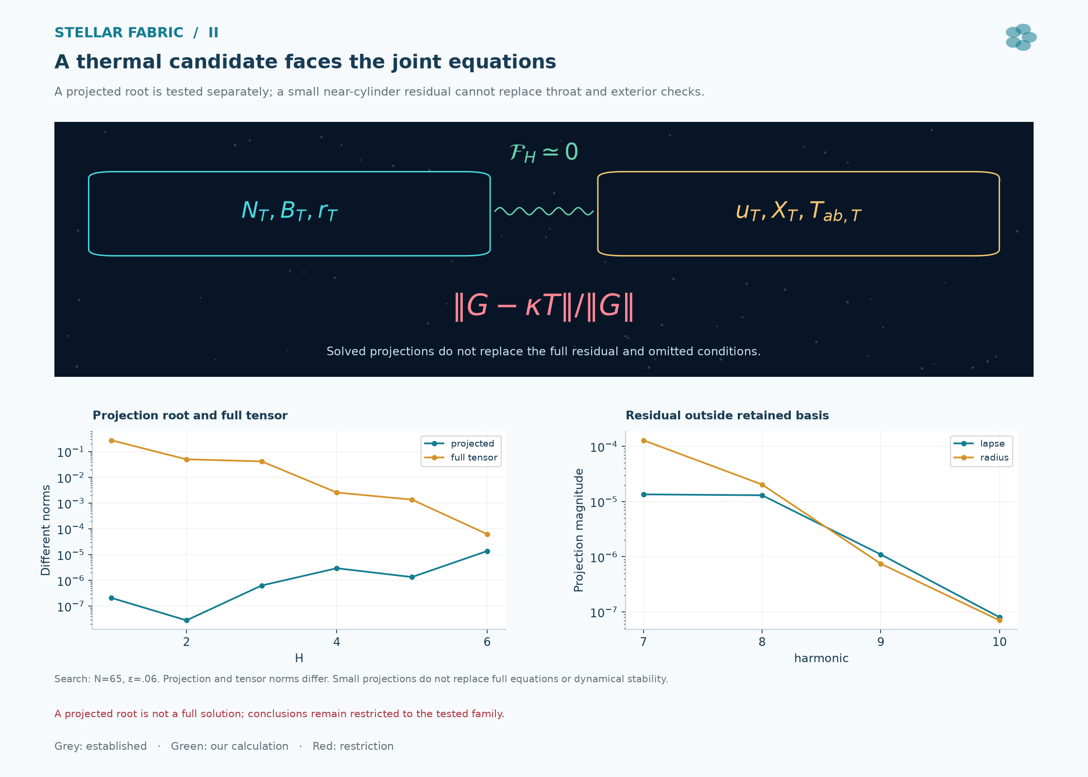
Tg=0.10546875, ε=0.06, 65 points, κ=3806.3838185. Retained-projection norm: 1.3741406×10⁻⁵. Full relative tensor residual: 6.2436981×10⁻⁵. No search bound is active.
Residual cross-check
Recomputing the residual from the three tensor components with the same κ gives the same value. This checks the arithmetic, not the physical assumptions.
Constant-radius control
A separate near-exact product control is retained separately. Its constant radius has no flaring minimum and is not evidence for a throat.
Derivation & model scope
Represent positive radius and lapse by exponentials of finite cosine series and include the constant length mode.
Recompute the thermal state and mean fields for each trial; a fixed old source is not carried into a new metric.
Solve the retained projected equations, then evaluate the unprojected three-component residual and the omitted Fourier content with the same κ.
The selected H6 point is a finite-regulator approximate stationary branch on closed S¹×S². It has not passed unprojected static closure, exterior completion, joint causal stability or loading. A small weighted residual is numerical evidence and has no certified interval error bound.
Agreement at one finite prescription does not establish a regulator-independent solution.
What remains unresolvedA controlled regulator prescription and the full field equations must be completed before physical source admission.
Keep the full tensor beside the projected rootWithin the declared finite prescription (65 radial nodes, epsilon=0.06), the nonconstant branch reduces its full tensor residual from 0.274 at H1 to 6.24 x 10^-5 at H6. The projected norm uses a different definition. Projections outside the retained basis remain separate checks. These bounded numerical results do not establish a complete physical solution or dynamical stability.Open full-size research figure ↗
07
Numerical accuracy
Grid accuracy does not settle regulator dependence.
Increasing spatial resolution at the selected cutoff leaves the best residual almost unchanged. Reducing the proper-time cutoff, while keeping geometry and κ fixed and re-solving the means, makes it larger. The two tests support different conclusions and must be shown together.
Established starting point
A covariantly subtracted quantum source still requires a controlled prescription for its finite inputs and regulator limit. Replacing a finite source by a claimed physical stress tensor needs more than agreement between two spatial grids. [4] [5]
What we derived or checked
We held the geometry and κ fixed while comparing spatial and cutoff refinements, and recalculated the source in each case.
(07.1)
Ngrid is spatial resolution, νmax and ℓmax the retained frequency and angular ranges. ε is the four-dimensional proper-time cutoff. The refinement table fixes the geometry, Tg and κ, and re-solves the retained means for each prescription.
Tests & outcome
Checks for result 07: Refinement is two different questions
Check
Result
ε=0.06 · 65 → 113 spatial points
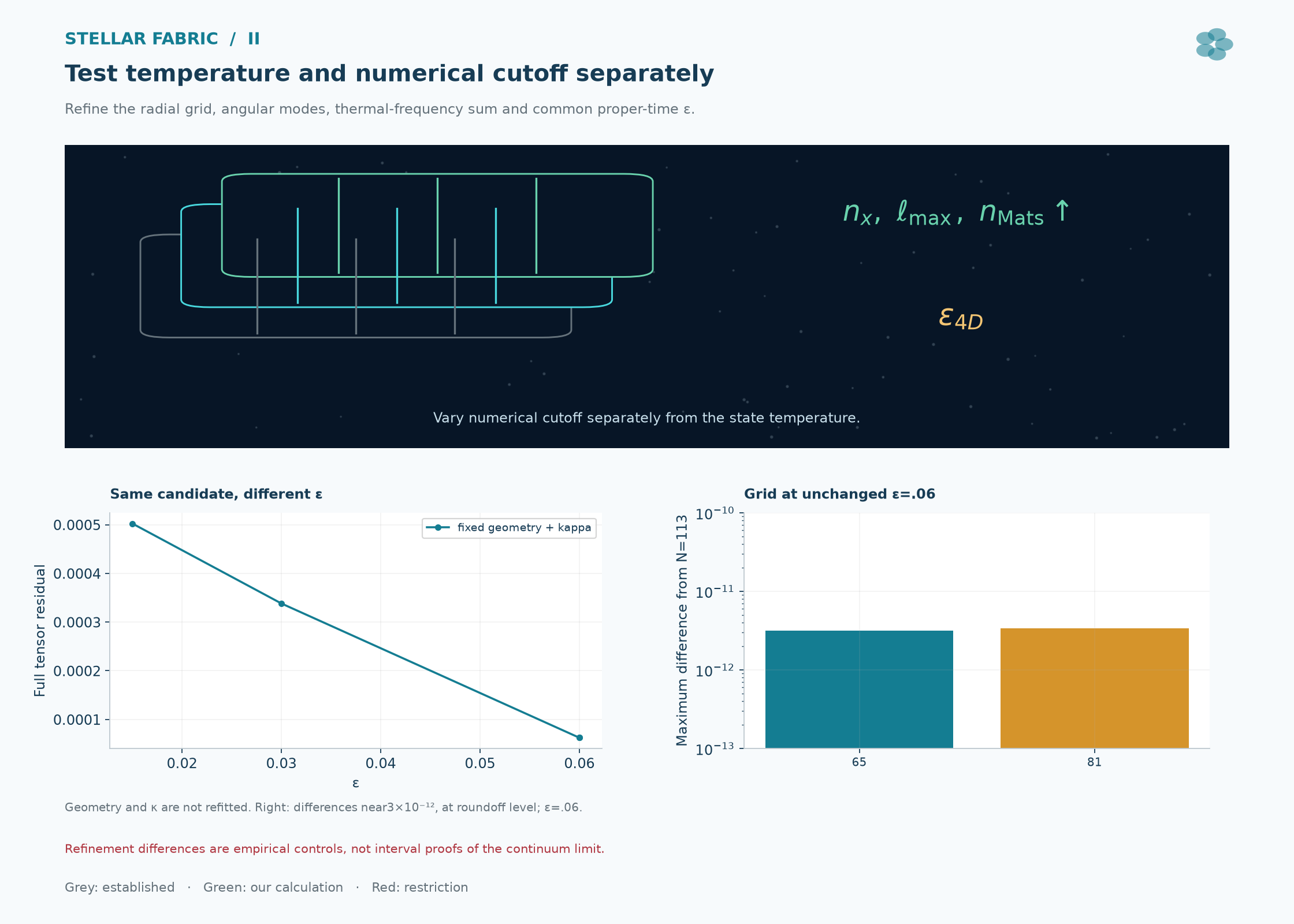
ℛfull: 6.2436981×10⁻⁵ → 6.2437131×10⁻⁵. This tests spatial accuracy at the same finite prescription.
ε=0.03 · re-solved means
ℛfull=3.3825455×10⁻⁴, at unchanged geometry and κ.
ε=0.015 · 145 spatial points
ℛfull=5.0243247×10⁻⁴. This is approximately 0.0502%, not the selected search residual of 0.00624%.
Derivation & model scope
First compare two spatial grids at fixed ε and otherwise matched inputs.
Then lower ε and recompute the mean state and stress while freezing the geometry and κ.
Report both changes. This sequence measures prescription sensitivity; it does not establish the ε→0 limit or the error of a physical apparatus.
Attaching exterior regions changes the operator, its spectrum, its state and its boundary-dependent source. The present periodic-cell source cannot simply be reused on that different geometry. Static positivity at fixed geometry likewise does not establish a joint retarded spectrum.
Both grid refinement and cutoff sensitivity matter when assessing the residual.
What remains unresolvedControlled renormalization, unprojected static closure, recomputed exterior matching, full dynamical stability, a finite maintenance budget and loading remain open.
The cutoff test changes the conclusion about accuracyChanging ε at fixed geometry and κ tests the finite prescription: the full residual rises from about 6.24×10⁻⁵ at ε=0.06 to 5.02×10⁻⁴ at ε=0.015. At unchanged ε=0.06, the 65- and 81-point sources are compared with the 113-point source on a common 257-point interpolation grid; the maximum tensor-component difference is about 3.40×10⁻¹². These are empirical numerical controls, not a proof of the continuum limit.Open full-size research figure ↗
THE NEXT SCIENTIFIC REQUIREMENT
A small residual is a starting point for harder tests.
The new branch needs controlled renormalization and completion of the unprojected static equations. Exterior matching must then recompute the boundary-dependent operator and source; attaching exterior regions to a periodic-cell solution changes the problem.
01
Close the static source.
Fix physical finite inputs and control the regulator prescription. Test all static components and constraints with the same source.
02
Let the whole system move.
Test the coupled retarded matter–geometry problem. A fixed-geometry matter bound or selected static harmonics do not give its full spectrum.
03
Account for preparation and use.
Specify the reservoir, control, heat removal, exterior and passage of a finite load. None has been physically validated here.
METHODS & SOURCES
The theory behind the calculation.
We compared cold and thermal states, checked their energy balance and tested how well the calculated stress fits the geometry. On one fixed geometry, heating made the total proper energy positive while the null stress at the minimum radius stayed negative. A separate search found a closer static match. The cutoff still affects the result, and full stability remains untested. The references below explain the theory behind these calculations.
Established separation of compactification and reference tensors in a different geometry. Result 02 uses an identical-cell comparator and includes its medium response.
Established common-action conservation framework. The project calculates the declared relative and thermal sources, without importing a complete solution.
Established covariant heat-kernel coefficients and subtraction tools. The declared project functional and its finite-prescription tests are separate calculations.
D. L. López Nacir, F. D. Mazzitelli & L. G. Trombetta · 2014
Antecedent for a renormalized stress tensor from a stationary effective action. Its Hartree/de Sitter solutions are not the project’s leading-order large-N periodic-product result.
Established Gaussian KMS and static Euclidean construction used in the fixed-background source approximation; not an existence theorem for the coupled project geometry.
Established relation of static effective actions, thermal energy and stress. Result 05 distinguishes the project’s Killing and proper-slice energy gates.
Established throat/null-energy requirement. The project’s periodic trial geometries and restricted thermal roots are not a complete traversable solution.