Stellar FabricWhat would it take to hold a wormhole open?
What states of matter and fields could support a traversable wormhole—and remain consistent when the system is disturbed or loaded?
By Stan Schneider
Reviewed
Research dossier · 10 results
Conceptual geometry · not a computed solution
THE RESEARCH QUESTION
The geometry is only part of the problem.
A traversable wormhole is a proposed connection between regions of spacetime through which matter or signals could pass. For a candidate to become physically meaningful, its supporting matter, boundaries and response to disturbances have to agree with the same laws.
Stellar Fabric studies the connection between a proposed spacetime geometry, the source that would support it, and the cost of keeping that source under control. The work combines analytical derivations with explicitly bounded numerical models. The results below follow that chain from source matching and constrained motion to state preparation and quantum stress.
In the Einstein-gravity throat framework studied here, the source must meet a negative null-stress requirement near the throat. Quantum theory also constrains negative energy. These are established starting points, not results invented by this project. [1][2]
RESEARCH STATUS · OCTOBER 15
The work has produced conditional mathematical results, numerical cross-checks and restrictions on candidate mechanisms. A stable physical wormhole and a realizable supporting material have not been established.
These calculations test geometry, supporting stresses, allowable motion and loading. A favorable result in one part of a system can coexist with a failure elsewhere. Those failures help narrow the next model.
FOCUS II
A source, its boundaries and its response
State preparation and response
Here we follow the source more closely: how a state is prepared, how the control fields react, what happens at the boundary and which stresses the geometry requires. These calculations use one specified interaction.
The ten entries below show selected derivations and their implications. The calculations use different stated approximations; their partial successes do not combine into a self-consistent loaded spacetime.
TEN RESULTS · EQUATIONS & CHECKS
Follow the calculation, not just the claim.
The first five results examine matching, energy and permitted motion. The next five follow one specified interacting seed. Each result shows the starting theory, what we calculated, how we checked it and what remains unresolved.
Notation is local to each result. The interacting-source calculations use normalized model units (c=ℏ=1); residuals describe the numerical tests, not certified error bounds. Exact finite-model identities and numerical evidence are labelled separately. Long equations scroll horizontally on small screens.
A traceless source does not complete the chosen two-ended geometry.
Conditional analytical obstruction
For the fixed spherical shape b(r)=r₀²/r, imposing a traceless Einstein source determines the lapse. The resulting family cannot stay positive and approach a nonzero finite value at both ends.
Established starting point
The input is the standard Einstein tensor and the zero-trace condition. Scalar-flat wormhole geometries are established in Dadhich and collaborators; their wider family is not excluded by this fixed-shape calculation. [7]
What we derived or checked
We solved the lapse equation for this chosen shape and checked the proposed source against the complete tensor, rather than matching only its negative radial component.
(01.1)
(01.2)
l is signed proper radial distance; r₀ is the throat radius; N is the positive lapse in gₜₜ=−N²; A and B are integration constants. Setting B=0 makes both end limits zero.
Tests & outcome
Checks for result 01: Two-ended source matching
Check
Result
Independent ODE integration
Runge–Kutta integration agrees with the closed lapse at maximum error 8.57×10⁻¹².
Two-end test
For B≠0 the limits have opposite signs. For B=0 neither limit is the required nonzero constant.
Derivation & model scope
Insert the fixed shape into the static spherical Einstein equations and impose vanishing source trace. In proper-distance coordinates the lapse equation has the displayed two-constant solution.
Take the two asymptotic limits before selecting constants. Their signs give the obstruction directly; numerical agreement checks the implementation, while the limiting argument establishes the restriction.
Scope: smooth, static spherical geometry, the specified shape, Einstein gravity and the stated two-ended lapse requirement. Changing the shape, source trace or asymptotic conditions is a different problem.
Tensor matching and lapse, checked by the closed-form solution and numerical integration.
What remains unresolvedA different compatible source and geometry are still needed. This is not a no-go theorem for all wormholes.
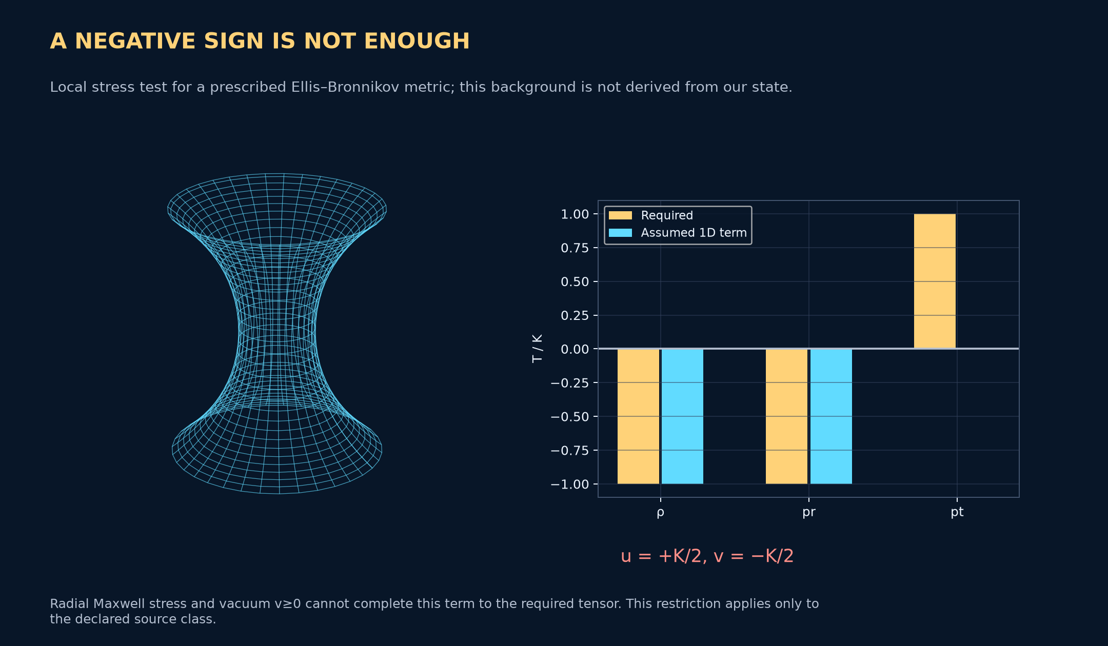
From a negative sign to the complete tensorThe wireframe is an embedding of the prescribed Ellis–Bronnikov geometry, not a geometry discovered or sourced by our state. The local comparison shows why the assumed one-dimensional term plus radial Maxwell stress and a nonnegative vacuum term cannot complete the required tensor. This auxiliary tensor test is distinct from the lapse proof above; other source classes are outside its exclusion.Open full-size research figure ↗
02
Geometry and source
Zero exterior mass does not remove the interior energy-density budget.
Conditional analytical lower bound
For a defined static spherical class, the proper-volume integral of negative energy density on one side has a nonzero lower bound whenever the asymptotic shape value lies below the throat radius.
Established starting point
The shape-function mass relation and volume measures are established GR tools. Visser, Kar and Dadhich study an integrated energy-condition measure; our E₋ is a different functional, so these statements are not contradictory. [8]
What we derived or checked
We derived a bound for the negative-density proper-volume integral and evaluated smooth screened profiles that can have a quiet exterior while retaining a large interior requirement.
(02.1)
E₋=∫max(−ρ,0)dVproper on one side, with ρ the local energy density; b∞=lim b(r). G and c retain their SI meanings. E₋ is not apparatus mass or preparation work.
Tests & outcome
Checks for result 02: Interior negative-density budget
Check
Result
Analytical class
Smooth static spherical profiles, 0≤b(r)<r outside the throat, b(r₀)=r₀ and b∞≤r₀.
Independent profile quadrature
At screening radius R=2r₀: E₋G/(c⁴r₀)=0.711921 for the cubic profile and 0.686443 for the quintic profile; both exceed the zero-exterior bound 0.5.
Derivation & model scope
Use the Einstein density relation to express the negative part of the density through downward changes of b(r). Proper volume adds the factor 1/√(1−b/r).
For the stated nonnegative-shape class this factor is at least one. The total downward variation is at least r₀−b∞, giving the bound without choosing a particular smooth profile.
The result excludes negative-shape exteriors, dynamic or nonspherical geometries, singular layers and modified gravity. The two profile values are examples within the declared class, not a search over all admissible sources.
Interior energy budget and miniature-source screening.
What remains unresolvedA physically preparable stress tensor remains missing; a small ADM exterior indicator does not identify one.
03
Autonomous control
A conserved-current direction escapes the leading fast drive.
Analytical identity in a restricted field class
In the selected shift-symmetric multi-field class, the homogeneous field velocities carry conserved currents. Those currents force one common direction to be blind to every time-dependent stiffness harmonic.
Established starting point
Autonomous dynamical stabilization and its stored-energy cost have prior literature, including Allahverdyan and Khalafyan. That mechanism motivates the control question; it does not provide our field-class identity. [9]
What we derived or checked
We isolated a conserved-current restriction that a leading fast-averaged stabilizer must respect, including mixed three-field examples.
(03.1)
V is the constant homogeneous field-velocity vector; J is its conserved shift-current vector; G(t)=−Paa at zero spatial derivatives is the spatial-gradient Hessian of the Lorentz-scalar P(XAB,uᵢ); Ḡ is its time average. K is the constant positive temporal Hessian. The temporary aA are spatial derivatives, unrelated to the radius a in the interacting-source model.
Tests & outcome
Checks for result 03: A direction the drive cannot stiffen
Check
Result
Mixed-field identity audit
Twelve mixed three-field fixtures: max |GV−J|=4.57×10⁻⁸; a separate stress-identity residual is 5.71×10⁻¹¹. These are numerical fixture residuals, not rigorous error bounds.
Leading averaged direction
Each drive harmonic annihilates V. After canonical normalization the corresponding direction is K¹ᐟ²V; the leading fast-drive stiffening vanishes there.
Derivation & model scope
The Lorentz-scalar dependence of P gives G(t)V=J on the constant-velocity background. Shift-current conservation then makes J constant in time.
Subtract the time average. Every oscillatory harmonic annihilates V; the leading quadratic fast-averaging correction therefore leaves the corresponding canonically normalized common direction untouched.
Scope: local shift-symmetric P(XAB,uᵢ), the specified homogeneous solution, a closed linear block, constant positive K and leading fast averaging. Mixing with additional modes, variable K, other couplings or higher-order corrections require separate analysis.
Conserved-current blind direction in the specified field class.
What remains unresolvedThe identity does not rule out every controller. It rules out treating this proposed drive as independent support in its blind direction.
04
Corrected boundary calculation
The corrected moving boundary has no overlap at the tested point.
An early thin-shell calculation admitted a candidate near γ=600. Recomputing radial and angular conditions with one consistent two-sided moving-junction geometry removed that window at the selected point.
Established starting point
The starting method is the established junction-condition treatment of dynamic thin shells, including conservation and momentum flux, as in Lobo and Crawford. [10]
What we derived or checked
We corrected the geometry used in our candidate boundary law and compared angular positivity with the selected positive radial acceleration response on the same configuration.
(04.1)
(04.2)
γ is the coefficient of the postulated surface operator −γ(div u)²/2, in the declared model units; it is not a Lorentz factor. ξ=l/r₀=0.215 identifies the inherited proper-coordinate anchor, with reference r₀=32. R=r/r₀, v=dR/dξ and f₊ is the assigned exterior metric coefficient. I is the pressure response to shell acceleration.
Tests & outcome
Checks for result 04: A corrected stability window
Check
Result
Angular condition
The corrected angular sector requires γ>379.558972.
Radial condition
The selected positive acceleration response I>0 requires γ<356.339152. The interval is empty; γ=600 fails this response condition.
Derivation & model scope
Use the same two-sided extrinsic geometry for the moving interface. Hold exterior mass and charge fixed in the radial derivatives; retain the surface conservation and flux terms.
Compare the fixed-round-surface angular positivity threshold with the positive radial acceleration-response bound at the same configuration. Neither condition by itself is a full coupled stability theorem.
This rejects the earlier tested window in the inherited static bulk branch, with local surface matter and a hypothetical foliation operator. The angular bound comes from a nonconstant phase mode on a fixed round surface. No coupled angular metric spectrum, physical cutoff or microscopic realization is supplied.
Corrected two-sided moving-junction calculation. The earlier result is retained as a correction.
What remains unresolvedA revised boundary interaction would have to pass the corrected conditions and have a realizable source law.
05
Constrained perturbations
A negative kinetic coefficient appears when the proper-length mode is released.
Restricted-sector analytical & numerical result
A positive fixed-boundary calculation can miss a permitted collective motion. In the selected local planar layer, solving the constraints and releasing the common proper-length mode exposes a negative reduced kinetic coefficient.
Established starting point
The lapse–shift decomposition and elimination of nondynamical constraints are standard methods. Gleyzes and collaborators provide related ADM/EFT methodology; their cosmological result is not the result claimed here. [11]
What we derived or checked
We kept the region’s proper-length response in the same constrained model and checked its short-patch coefficient against the numerical reduction.
(05.1)
(05.2)
The radial metric scale is B=exp(b), the region’s length is ℓ=∫B dx, and the normalized length coordinate is qℓ=√(2L)b. Its reduced kinetic term is Jℓ q̇ℓ²/2. L is the half-width. βℓ is the positive higher-derivative coefficient, unrelated to the coupling β in the interacting-source model. Jraw is the unconstrained kinetic integral; C is the shift quadratic form and D its coupling to length velocity (these are not the covariance variables of that interacting-source model).
Tests & outcome
Checks for result 05: Let the region’s length respond
Check
Result
Background constraint control
On |x|≤0.08, the local background has maximum constraint residual below 2.57×10⁻⁹.
Reduced length sector
On [−0.03,0.03], Jℓ=−2.16791331 in the declared normalization. The analytical short-patch limit gives the same negative sign.
Derivation & model scope
Allow the proper length of the geometric region to vary along with the stated layer variables. Solve the lapse and shift constraints before reading off the sector’s reduced kinetic form.
Project to the declared common-length sector. The short-patch expansion has a negative leading coefficient; the finite-patch constrained reduction gives the quoted value.
The model is local and planar, with anchored induced lapse/transverse scale and zero endpoint shift, while proper length is free. The inherited higher-derivative term is −βℓ Aφ¹² Ktrace²/(2N⁶), where Aφ is the selected field amplitude. The finite projection and constitutive choice are restricted. This does not classify the full continuum or prove a global gravitational ghost theorem. The length is a geometric variable; no physical hardware support is identified.
Reacting local layer and proper-length calculation.
What remains unresolvedA favorable fixed-support result must be replaced by a compatible model of the allowed joint motion.
06
Same-action identities
A constant field normalization cannot lower the signal frequencies by itself.
Exact field identity & independent finite checks
For the specified positive normalization Z=Zref exp(βη), changing a constant Z scales both signal inertia and stiffness. Canonical normalization cancels this common factor. Gradients and time dependence contribute through the effective operator.
Established starting point
Field redefinition, integration by parts and boundary variation are established methods. Hollands and Wald supply conservation context; Ishibashi and Wald explain why the operator’s boundary law must be specified. [4] [3]
What we derived or checked
We derived the effective operator for the chosen η–χ–φ action, kept its boundary reaction, and tested the force identities in an independent spectral representation.
(06.1)
(06.2)
(06.3)
φ is the signal with mass parameter Mφ, χ and η are classical mean fields in this approximation, and Zref>0 is the reference normalization. h and β are couplings; U is the canonical quadratic effective mass term. □ and ∇ use the assigned spacetime metric.
Tests & outcome
Checks for result 06: What normalization can change
Check
Result
Exact identity audit
The polynomial checks of the canonical transform and variational force identities have zero residual coefficients.
Boundary force balance · N=32 fixture
Interior stationary η force −2.00585245×10⁻⁶ is cancelled by endpoint reaction +2.00585245×10⁻⁶; net uniform-shift force is 1.43×10⁻¹⁸.
Derivation & model scope
Insert φ=ψ/√Z in the quadratic signal action, expand its derivatives and integrate by parts. Keep the induced boundary term together with U.
For constant η and χ, the common Z cancels from the same-domain curved-space eigenproblem. In the homogeneous flat-space limit this gives ω²=k²+Mφ²+hχ. The uniform stationary η-force cancellation must include the endpoint reaction.
This restricts the constant-background normalization mechanism of the selected action. It does not exclude effects of varying η, a different coupling or boundary work. A full interacting renormalized source and physical boundary apparatus remain separate requirements.
Canonical normalization, exact identities and an independent spectral cross-check.
What remains unresolvedAn independent physical advantage from the proposed normalization has not been established.
07
Two-route quantum check
The vector edge tower restores the chosen ultraviolet calculation.
Established boundary formalism · project consistency result
On the fixed Euclidean product H²×S², counting only propagating vector bulk modes misses a harmonic boundary contribution. Including the full edge tower makes our local and spectral heat-kernel routes agree.
Established starting point
Vassilevich gives the standard local heat coefficients. Banerjee, Gupta and Sen, and Larsen and Lisbao establish the vector boundary-mode and product-space accounting used here. [12] [6] [13]
What we derived or checked
We applied that formalism to the selected mixed field seed, with its unequal product radii, and reconstructed the same ultraviolet coefficient by a second spectral route.
(07.1)
K is the local heat-kernel density, s is proper time, a is the H² radius, and R is the S² radius. The convention is Keff(s;x,x)∼(4πs)⁻²[a₀+a₂s+a₄s²+…]. Both routes use the same retained benchmark parameters and operator/ghost normalization. a₂ and a₄ name local short-time coefficients, not the radius a.
Tests & outcome
Checks for result 07: Complete the boundary sector
Check
Result
Independent a₄ routes · selected benchmark
Local: 1.080769540509. Spectral cubic extrapolation: 1.080769541522. Difference ≈1.01×10⁻⁹ in model units; this is not a certified error interval.
Domain and tail controls
Four uncoupled radius-pair fixtures agree to ≤4.45×10⁻¹⁶; independent quadrature/tail controls differ relatively by ≤2.30×10⁻¹⁶ at the tested proper times.
Derivation & model scope
Put the coupled local Hessian in Laplace form and include the gauge/ghost traces. Compute the local coefficient matrices.
Independently sum the physical angular towers and add the established H² harmonic one-form density times the full S² scalar tower. A separate true-zero-mode subtraction changes a₄ and requires its own measure.
This is fixed-product Gaussian ultraviolet consistency. It is not the full finite absolute stress tensor. Numerical extrapolation uncertainty, physical wall/exterior, charge ensemble, zero-mode measure and finite effective-action coefficients are not resolved by this match.
Product heat kernel and independent vector-edge check.
What remains unresolvedThe boundary sector is necessary accounting, not an identified supporting source.
08
Finite preparation and reserve
The correlations can be prepared through an explicit interaction.
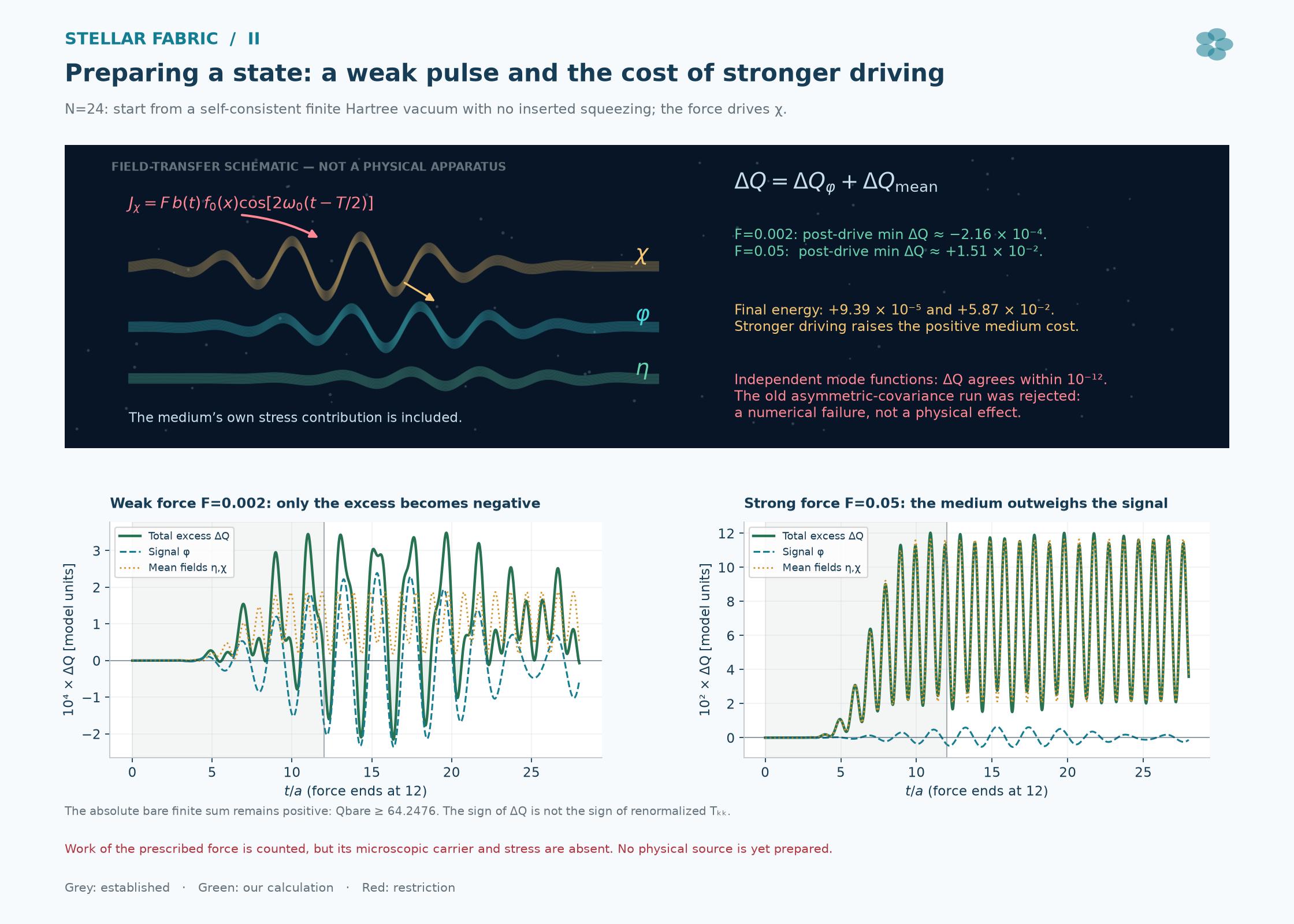
Starting from a finite self-consistent equilibrium, a χ-field pulse prepares signal correlations through a trilinear interaction. A separate run begins with a finite initial energy reserve and evolves without continued forcing. Both include the mean fields’ own contribution. The negative changes below are relative to the reference state; the absolute bare null observable stays positive.
Established starting point
Trilinear pair preparation and a stabilizing quartic potential have direct antecedents in Dufaux and collaborators. The standard mechanism is not a project invention. [5]
What we derived or checked
We combined reciprocal mean-field response, work accounting, total-null histories, independent mode-function controls and parameter ablations in the assigned curved radial domain.
(08.1)
(08.2)
These equations describe the separate closed-reserve run: M₀ is its positive mass matrix, F its normalized kick profile, A the initial amplitude and Jχ the external force. The driven comparison below uses a different force amplitude f₀. Numerical quantities are dimensionless model units, not joules or laboratory times.
Tests & outcome
Checks for result 08: Prepare a state and count the work
A=0.002 gives ΔE(0)=2×10⁻⁶ and minimum ΔQ=−3.40634×10⁻⁵. Energy drift ≤1.46×10⁻¹¹; independent total-null-history difference ≤1.51×10⁻¹².
Ablations and stronger drive
Removing h and λ disconnects the signal. Removing β leaves the weak-reserve minimum almost unchanged. At external f₀=0.05, post-drive minimum ΔQ is positive: +0.015094.
Derivation & model scope
A smooth external χ force changes the signal operator through hZχφ²/2. Evolve the covariance and both means, and count work as W=∫Jχᵀχ̇ dt.
Reconstruct the state independently with complex mode functions. For the separate closed-reserve case, change only the initial χ momentum; its positive quadratic kinetic cost is A²/2.
Hartree approximation: Gaussian signal, classical χ and η, assigned geometry and boundary law, finite grid and finite test durations. ΔQ=Qbare−Qequilibrium is a reference-state change. The absolute bare Q remains positive in both runs. A microscopic force carrier and preparation of the initial kick are unresolved.
Driven preparation, closed-reserve evolution and independent mode-function checks.
What remains unresolvedThe run demonstrates finite-model preparation, not a physical negative source or autonomous wormhole maintenance.
State preparation, with the medium includedThe upper waves are a field-transfer schematic; the lower curves are computed N=24 finite-Hartree histories. The panels use different vertical scale factors (10⁴ and 10²). Their common ΔQ is a reference increment, not absolute renormalized null stress. Work, mean-field response and the rejected numerical failure are kept explicit.Open full-size research figure ↗
09
Analytical finite-model result
A square completion gives an exact bound for the closed finite model.
Exact finite-model theorem · no continuum claim
With positive masses and the specified coupling relation, the Hartree potential can be written as a positive square plus a positive remainder. Conserved absolute energy then bounds the finite variables and the selected bare null observable.
Established starting point
Square completion, symplectic covariance transport and finite-dimensional ODE continuation are standard mathematics. The underlying trilinear/quartic potential has established preheating antecedents. [5]
What we derived or checked
We derived the Hartree remainder, explicit sitewise energy bounds and the positive-window null budget for this same closed finite action.
(09.1)
(09.2)
(09.3)
C=⟨φ²⟩ is the local signal variance in the zero-mean Gaussian sector; λ=h²/(2mχ²). Eabsolute includes the finite vacuum contribution. Qnull uses finite bare stress with window weights between zero and one, including both endpoints of that range.
Tests & outcome
Checks for result 09: An exact finite energy theorem
Check
Result
Exact algebra
Six sparse-polynomial identities have zero residuals, including square completion, energy cancellation, the symplectic generator and the null budget.
What establishes the theorem
Energy inequalities and finite-dimensional continuation give the exact result. No new trajectory or numerical evaluation of the bound was used as its proof.
Derivation & model scope
Complete the potentially negative cubic term together with the positive quartic and χ-mass terms. Remaining kinetic, gradient, mass and magnetic energy terms are nonnegative.
Conserved Eabsolute bounds η, hence both Z and 1/Z, as well as variances, momenta and off-diagonal covariances. The exact symplectic flow preserves quantum physicality. The smooth finite ODE therefore cannot blow up in finite time.
The radial magnetic and potential contributions vanish in the null contraction. The remaining positive terms give the displayed budget. A larger kick cannot reverse this finite bare sign.
Fixed finite grid, time-independent boundaries, physical initial covariance, positive coefficients and exact autonomous equations. This proves no finite-time blowup, not closeness to equilibrium. The bound depends on cutoff and absolute finite energy; it is not a uniform continuum, full gravitational-stability or renormalized-sign theorem.
Exact coercivity and the raw-null energy budget.
What remains unresolvedThe sign of a covariantly renormalized stress requires physical subtraction and matched finite terms. It is not determined by the positive bare bound.
10
Necessary geometric condition
A shallow throat still needs the correct first-order source response.
Expanding around the constant-radius product makes the source requirement precise. A small localized flare asks for a signed first-order null stress, while the declared classical positive-kinetic sector has no linear null contribution there.
Established starting point
The relation between flaring geometry and null stress is established by Hochberg and Visser. Our calculation specializes that requirement to the selected product background and its allowed source response. [1] [4]
What we derived or checked
We derived the normalized first-order equation, checked its contact and counterterm signs, and evaluated the spatial sign pattern of the chosen localized test direction.
(10.1)
(10.2)
ds²=−exp(2Φ)dt²+dx²+r²dΩ², r=R(1+εu), Φ₀=log cosh(x/a), and k=(exp(−Φ),1,0,0). Primes denote x derivatives. Gkk and Tkk are contractions with this metric-normalized radial null vector; ε is the small flare amplitude.
Tests & outcome
Checks for result 10: Match the actual geometric demand
Check
Result
Exact first-order audit
Eight exact rational-polynomial checks have zero residuals, including Gkk, the zero classical linear term and varied-null-vector contact cancellation.
Localized test profile
u=−sech²(x/4a) gives (δGkk/ε) at x=0 equal to −1/(4a²); its sign changes at |x|/a≈1.049914.
Independent integral checksum
A 4096-panel Simpson check differs from the closed-form weighted integral by 2.43×10⁻¹⁶. This checks an identity, not physical source admission.
Derivation & model scope
Contract the spherical Einstein tensor: Gkk=−2(r″−Φ′r′)/r. Linearize about constant r=R to obtain the displayed operator on u.
Classical scalar-gradient squares start at order ε² on the constant-field background; potentials drop out of the null contraction and radial magnetic null stress is zero.
The necessary branch equation is [L−(κ/2)Πeff]u=0, where Lu=Φ₀′u′−u″, κ=8πG/c⁴ and Πeff is the matched quantum and local-term response. ε cancels. Reducing the flare alone does not repair an incorrect response coefficient.
This is a necessary radial condition, not the complete tensor equations. The full renormalized response Πeff was not computed, no operator norm was established, and the semiclassical background was not closed. The absence of a localized solution to Lu=0 does not prove a uniform gap on the infinite line.
First-order product-branch requirement and localized sign check.
What remains unresolvedA physically specified source, boundary/exterior and finite effective-action coefficients must satisfy this equation together with the remaining field and constraint equations.
THE NEXT SCIENTIFIC REQUIREMENT
Bring the source and its response into one physical model.
The next task is a consistently defined interacting source, its quantum state, boundary and exterior, with a physically specified prescription for finite quantum stresses. Geometry and loading then have to be tested with that same source.
Success requires compatible answers to all five questions below. A positive result for one sector cannot stand in for the whole system.
01
Existence
Do geometry, matter, boundaries and the exterior solve one compatible set of equations?
A complete physical throat solution remains open.
02
Perturbations
What happens when the source, support and geometry move together?
Selected sectors are tested; full joint stability remains open.
03
Loading
Does the candidate survive finite matter or energy passing through it?
Partial loading tests do not establish sustained passage.
04
Maintenance
What supplies control, reaction time, work and heat removal?
A physical actuator and complete operating budget remain open.
05
Physical source
Can the required stress be produced, prepared and measured?
A realizable supporting source has not been established.
METHODS & SOURCES
The literature and the project calculation.
We tested how proposed sources match the geometry, examined their allowed motion and followed how a state could be prepared. Analytical derivations and numerical cross-checks show where the chosen models work and where they fail. They do not yet establish a physically realizable supporting material or a stable wormhole. Scientific priority has not been established; the references below identify the established theory behind the calculations.
Established integrated energy-condition measures. Result 02 uses a negative-density proper-volume functional and a narrower profile class, not the same measure.