Stellar FabricOther approaches to the quantum source

ALTERNATIVE APPROACHES

What changes when we change the model?

We broadened the search to fermionic vacuum sources, their sustaining fields and a quantized gauge phase. The calculations give useful restrictions and a conditional negative contribution. We also checked a more practical issue: whether an accurate energy calculation actually gives an accurate stress. One finite-model example fails that test; a different choice of reduced states improves static response substantially. Each result below keeps its own state, action and boundary conditions.

The previous update tested how a chosen source matches a prescribed geometry. Its calculations remain available with their original assumptions.

7 FINDINGS · EQUATIONS & CHECKS

The calculation and what it tells us.

Each result shows what we changed, what we calculated and which questions the answer leaves open.

Notation and units are defined for each result. Numerical checks apply to the stated model and approximation. Long equations scroll within their own blocks on small screens.

1. 01A bound covering every smooth profile
2. 02Ask what sustains the mass profile
3. 03Quantize the phase and check the sign
4. 04Check the stress separately from the energy
5. 05Keep the second metric derivative
6. 06Choose reduced states for the quantity being tested
7. 07Separate thermal redistribution from isolated response

01

Fermionic vacuum

Changing the mass profile has a definite energy cost.

Analytical result · flat antiperiodic vacuum · fixed RMS mass

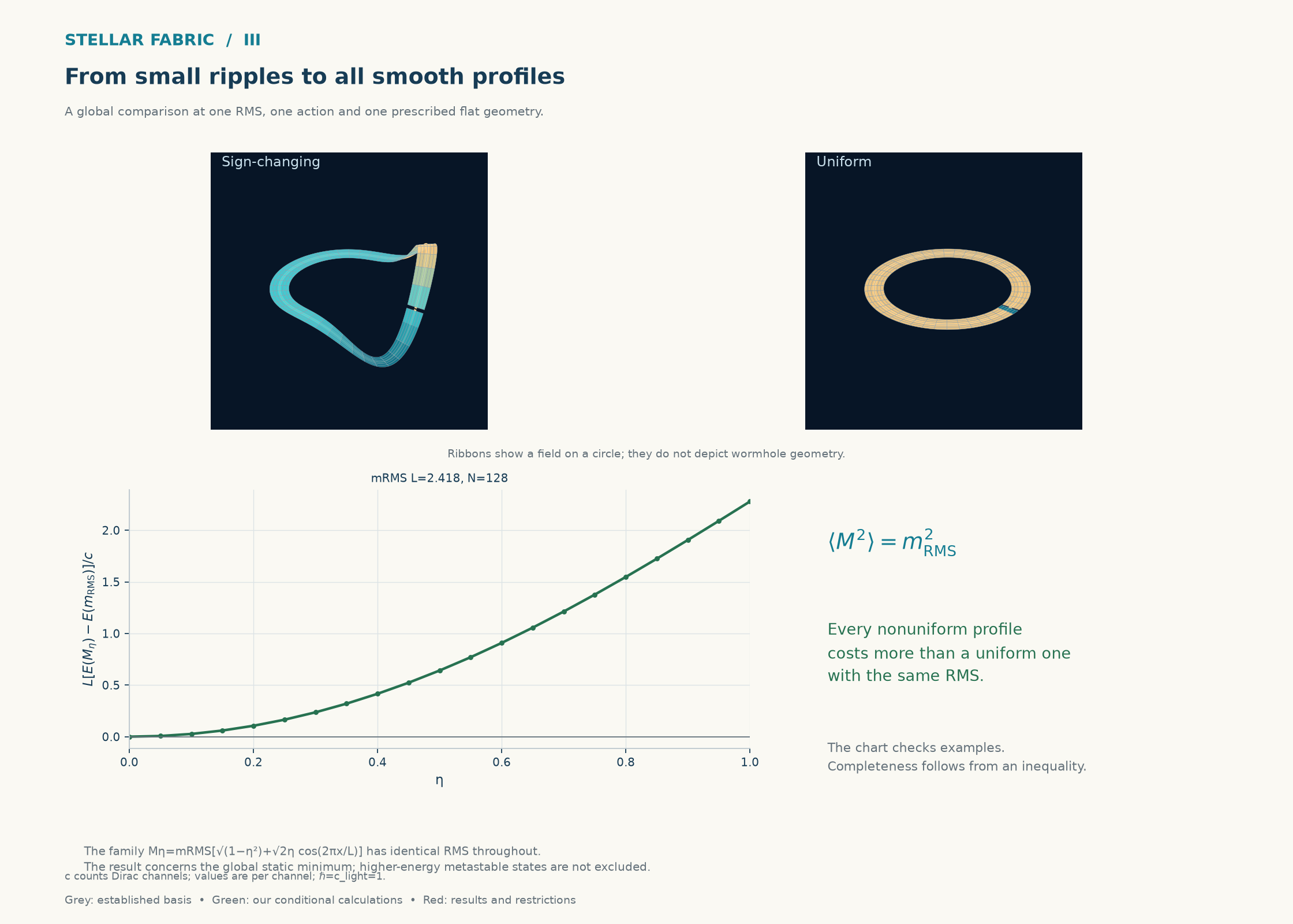
We compared a varying real mass with a uniform field of the same root-mean-square mass. For the stated vacuum and carrier action, every smooth nonconstant profile costs more total energy. The conclusion covers the whole declared class, rather than only the shapes in a numerical search.

Established starting point

Operator Jensen inequalities and renormalized Dirac vacuum energies are established tools. Inhomogeneous fermion states are also known; their charge, topology and state constraints can differ from this vacuum problem. [1] [2] [3]

What we derived or checked

We combined a translation average of the squared Dirac operator with cancellation of the common mass-squared subtraction. A separate resolvent argument confirms the vacuum-energy sign.

$$E\left[M\right]-E\left[m_{\text{RMS}}\right]\ge \frac{\kappa }{2}\int {\mathrm{M\prime }}^2\mathrm{dx}+\frac{u}{4}\int {(M^2-s)}^2\mathrm{dx}\ge 0$$

(01.1)

Here s=L⁻¹∫₀ᴸM²dx and mRMS=√s. Integrals run over the flat circle of circumference L. κ>0 is the carrier gradient coefficient, not a gravitational coupling; u≥0 is its quartic coefficient. One complex Dirac channel has antiperiodic boundary conditions, zero temperature and zero chemical potential.

Tests & outcome

Checks for result 01: A bound covering every smooth profile

Check	Result
Scope of the proof	All smooth real periodic profiles for which the uniform equal-RMS comparator is admissible. No finite profile scan supplies the completeness claim.
Numerical controls	Seven profile families, three RMS values and four cutoffs. The largest observed change between the two finest retained cutoffs was 3.78×10⁻⁴ in dimensionless relative energy per channel; it is not a total error certificate.

Derivation & model scope

1. Translation-average the squared Dirac operator; its mean mass term is s and its derivative term averages to zero.
2. Apply the trace inequality, retain the same renormalization, and add the nonnegative gradient and quartic costs.

The comparison uses a free-fermion determinant and a classical carrier, without carrier loops. Curvature, complex masses, finite density and constraints excluding the constant comparator change the problem.

The project result is this global comparison for the specified vacuum action.

What remains unresolvedThe bound does not exclude higher-energy metastable profiles, order their null stress or prove dynamical stability.

02

Carrier consistency

An exactly massless core fails the chosen autonomous field equation.

Local determinant variation · canonical Yukawa carrier

We tested a field that makes one part of a compact channel massive while leaving an open interval exactly massless. The vacuum still exerts a nonzero force inside that interval. The proposed profile therefore fails the stationary equation of the selected autonomous carrier.

Established starting point

Dirac vacuum condensates and self-consistent scalar backgrounds are established. A prescribed mass profile must also satisfy its carrier equation if it is to persist without a specified external controller. [2] [3]

What we derived or checked

We varied the full-circle vacuum energy locally, determined the sign inside the zero-mass interval, and inserted that source into the same-action Yukawa equation.

$$-\mathrm{Z\phi ″}+\mathrm{U\prime }\left(\phi \right)+\mathrm{y𝒞}=0\text{;}{\phi }_{\text{core}}=0\Rightarrow \mathrm{y𝒞}\ne 0$$

(02.1)

M=yφ and 𝒞(x)=δEψ,ren/δM(x). The chosen flat antiperiodic vacuum has a bounded real nonnegative return mass, nonzero on a set of positive measure. Z>0, y≠0, and the position-independent even potential obeys U′(0)=0. Under these assumptions, 𝒞(x)<0 throughout the open core.

Tests & outcome

Checks for result 02: Ask what sustains the mass profile

Check	Result
Local versus full-energy variation	Eighteen signed compact probes agreed with the integrated local source to within 6.59×10⁻⁹ per channel in the numerical comparison.
Smooth returns	Twelve smooth return profiles, each with six refinements, retained the nonzero core source. The selected transfer refinement changed source/pressure by at most 6.55×10⁻⁸; this is not a bound on every numerical error.

Derivation & model scope

1. Use transfer positivity to determine the local condensate inside the exact-zero interval.
2. There φ and its derivatives vanish, leaving y𝒞 as an uncancelled term in the carrier equation.

The restriction concerns this canonical autonomous construction. A small nonzero core, another state, additional interactions or an external controller require separate tests.

Matching a pressure at a boundary does not, by itself, make the field profile stationary.

What remains unresolvedThis does not exclude the different Maldacena–Milekhin–Popov mechanism or all fermionic sources. No four-dimensional source or coupled geometry is solved here.

03

Quantum source candidate

A quantized phase retains a conditional negative null contribution.

Specified winding-potential effective model · fast matter held in vacuum

We promoted a compact gauge phase to a quantum rotor and calculated its equilibrium state. In this effective model, the longitudinal null combination remains negative at every finite rotor temperature. The condition is essential: the matter that creates the winding potential stays in its vacuum.

Established starting point

Gauge phases, winding vacuum potentials and positivity of thermal operators are established ideas. We applied them with an explicit geometry-dependent rotor inertia and a declared ensemble. [4]

What we derived or checked

Positive winding coefficients and nonnegative cosine means give an analytical sign argument. We evaluated the corresponding quantum and thermal rotor states separately from the finite bare matter model below.

$$E_w=-{\sum }_{w\ge 1}{a}_w\cos \left(\mathrm{w\theta }\right)\text{;}{𝒩}_L=U-D_{L}F=-{\sum }_w(a_w-D_L{a}_w)⟨\cos \left(\mathrm{w\theta }\right)⟩<0$$

(03.1)

DL=∂lnL at fixed physical inputs; aw>0 and DL aw<0. U is internal energy and F free energy, not a scalar carrier potential. 𝒩L is the integrated energy-plus-longitudinal-pressure combination; L is a circumference. Units are ℏ=c=kB=1. The compact U(1) field is auxiliary, with charge 9, not ordinary electromagnetic charge. The rotor inertia is Iη=4πKauxR²/L, with fixed positive Kaux.

Tests & outcome

Checks for result 03: Quantize the phase and check the sign

Check	Result
Quantum and thermal evaluation	Thirty-six model choices and 1620 thermal states support the declared sign. The argument also covers positive mixtures of the nine preserved residue sectors.
What is being heated?	Only the slow rotor is thermal. Excitation of the matter field, a physical reservoir and preparation of the sector weights are not included.

Derivation & model scope

1. Retain the same free-vacuum potential while quantizing the phase and its electric kinetic term.
2. Differentiate the canonical inertia with geometry; its direct longitudinal null contribution cancels, leaving the winding sum.

The exact ultrastatic product requires zero total longitudinal null combination. A negative rotor contribution alone therefore does not solve its Einstein equation. This effective model and the later bare finite model have not been matched into one renormalized source.

The sign is a conditional result for this effective model; it cannot be added to a different vacuum calculation without matching them.

What remains unresolvedA negative contribution is not yet a complete supporting material, a heated quantum-field state or a stable wormhole.

04

Physical metric work

A good energy estimate can hide a poor stress estimate.

One finite Hamiltonian · moving trial spaces

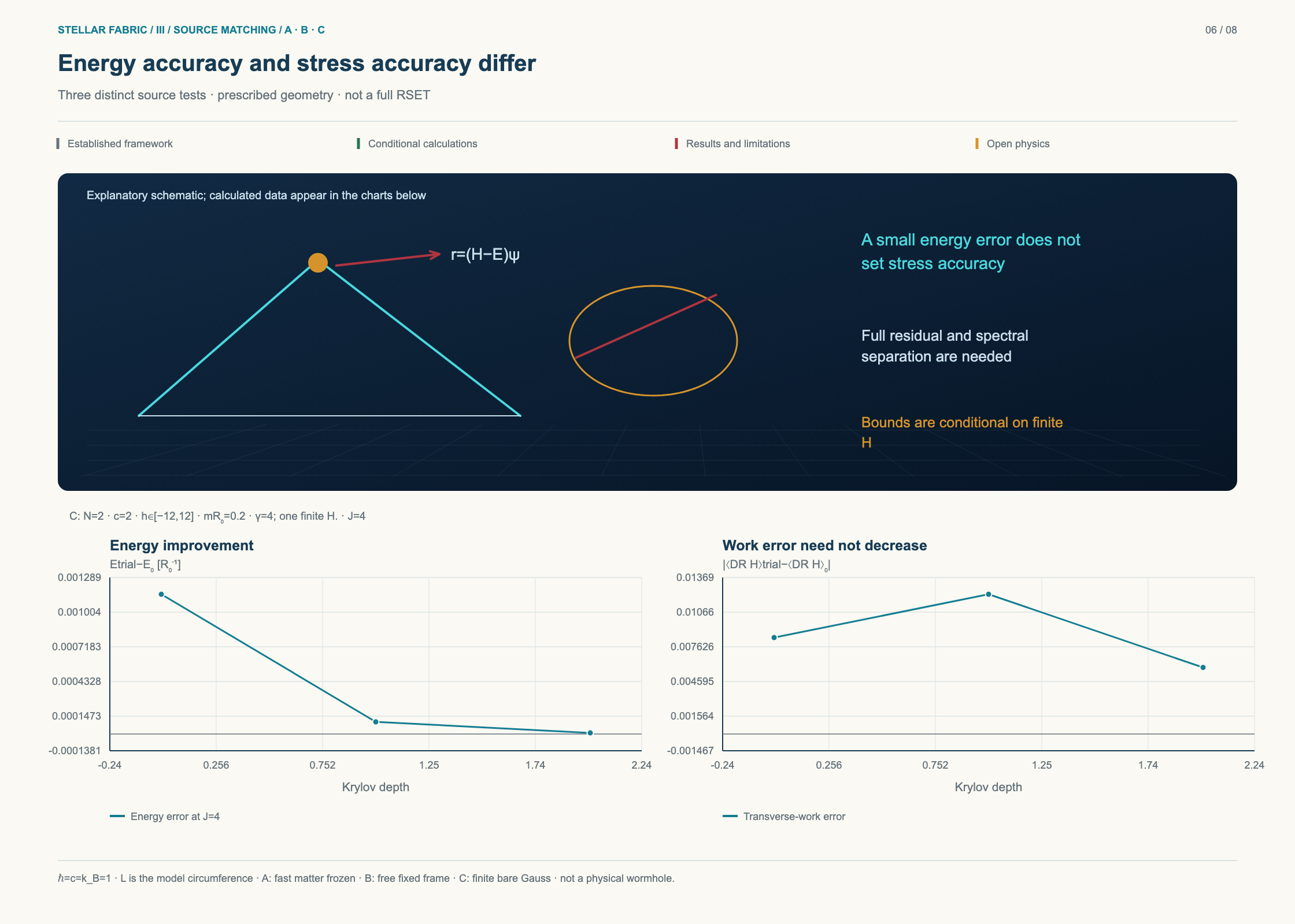
We found a case where improving the energy made the transverse metric work less accurate. The derivative of the approximate energy looked convincing because motion of the trial space compensated for the physical-work error.

Established starting point

The variational derivative contains the established Pulay correction when the trial space changes with geometry. [5]

What we derived or checked

We separated the two terms and compared the physical work with the exact finite reference.

$$D_y{E}_{\text{trial}}=⟨D_{y}H⟩+2\mathrm{Re}⟨D_y\psi |r⟩\text{;}r=(H-E_{\text{trial}})\psi$$

(04.1)

H is the finite Hamiltonian, ψ the normalized trial state, r its residual and y=ln R here. Metric work is an integrated stress quantity, not a local pressure.

Tests & outcome

Checks for result 04: Check the stress separately from the energy

Check	Result
Energy versus work	Energy error fell about 11.5 times, while the transverse-work error grew about 45%.
Compensating terms	Physical work −0.0212541 versus reference −0.0334755: 36.5% error. Adding Pulay −0.0122170 gives the apparently accurate derivative −0.0334712.

Derivation & model scope

1. Differentiate the normalized trial-state expectation and retain its full residual.

The decomposition agrees with finite differences to about 10⁻⁹ in this example. This and the next three results use one finite bare scalar/compact-U(1) Hamiltonian with exact local Gauss law on a prescribed ultrastatic time×S¹×S² product, L=6R₀ and R=R₀. Units are ℏ=c=kB=1; energies and metric work are in R₀⁻¹. The auxiliary charge is 9 and ordinary electromagnetic charge is zero. It is a separate model from the negative winding effective source.

Pulay work explains the cancellation. It supplies no additional physical energy.

What remains unresolvedThe reference is a finite matrix; accuracy in the full field theory remains unproved.

05

Geometry and response

The mixed metric contact recovers a missing component.

Four operator components · fixed physical parameters

Our Hamiltonian contains four components. Energy and its two first metric derivatives recover only three independent combinations. The mixed second derivative supplies the fourth, allowing the reduced calculation to retain information that energy alone misses.

Established starting point

Established linear response combines a direct change of the operator with the change of its quantum state. [6] [7]

What we derived or checked

We derived both terms from the same finite Hamiltonian and checked their sum against metric differences.

$$H(x,y)=e^{-x-2y}{T}_{\text{kin}}+e^{x+2y}B+e^{-x+2y}{V}_{\text{grad}}+e^{x-2y}{E}_{\text{el}}$$

(05.1)

$$S_{\text{LR}}=2(T_{\text{kin}}+B-V_{\text{grad}}-E_{\text{el}})$$

(05.2)

$$V_a={\partial }_{a}H\text{;}{S}_{\mathrm{ab}}={\partial }_a{\partial }_{b}H\text{;}{K}_{\mathrm{ab}}=⟨S_{\mathrm{ab}}⟩+{\chi }_{\mathrm{ab}}$$

(05.3)

x=ln(L/L₀), y=ln(R/R₀); a,b label these metric variations. The four terms are evaluated at the reference geometry: matter kinetic Tkin, mass B, spatial gradient Vgrad and electric-flux Eel. The displayed SLR identity is at x=y=0. Physical mass, gauge coupling, canonical anchor and finite embedding are held fixed. χ is the state response; K is the isothermal kernel here.

Tests & outcome

Checks for result 05: Keep the second metric derivative

Check	Result
Component information	Adding SLR raises the coefficient rank from three to four; the resulting determinant is −64.
Metric differences	Maximum normalized discrepancy: 9.31×10⁻⁶ for diagonal checks and 1.81×10⁻⁶ for mixed checks.

Derivation & model scope

1. Differentiate at fixed physical parameters, canonical operators and finite embedding.

This identity closes four component combinations, not the quantum state space.

The contact is part of the response, not a separate force.

What remains unresolvedSpatial perturbations, the complete stress tensor and coupled gravitational dynamics remain outside this calculation.

06

Reduced quantum calculations

States selected for stress gave a better static response.

Thirty-six comparisons · equal retained dimension

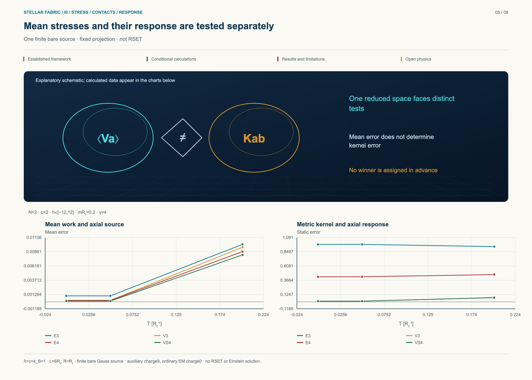
We compared an energy-based Krylov space with one built from energy and physical metric-work operators. At the same retained dimension, the latter improved static response in every tested model–temperature pair, although mean stresses did not always improve.

Established starting point

Krylov reduction is established. The question was which operators should select the retained states. [8] [6]

What we derived or checked

All methods used the same finite Hamiltonian and reference, with the reduced space held fixed during metric variations.

$$E_3=\mathrm{span}\{W,\mathrm{HW},H^{2}W,H^{3}W\}\text{;}{V}_3=\mathrm{span}\{W,\mathrm{HW},V_{L}W,V_{R}W\}$$

(06.1)

$${\epsilon }_K=\frac{\max |K_{\text{red}}-K_{\text{full}}|}{1+\max \left|K_{\text{full}}\right|}$$

(06.2)

W is the ground-band seed; E3 and V3 both retain 36 directions. Errors use fixed model units. The cohort includes twelve prescribed choices of lattice size, occupation cutoff, mass and coupling, at TR₀=0, 0.05 and 0.2; the full reference remains finite.

Tests & outcome

Checks for result 06: Choose reduced states for the quantity being tested

Check	Result
One zero-temperature example	Kernel error fell from 1.0352 to 0.0098936, a factor of 104.63, while the energy error increased.
Across the cohort	Static response improved in 36/36 comparisons; combined mean-stress error worsened in 8/36. Only 9/36 V3 static results meet the 0.001 accuracy criterion.

Derivation & model scope

1. Compare each reduced result with the same full finite reference.

These comparisons cover twelve models at three temperatures.

A large improvement can still leave an unacceptable error.

What remains unresolvedThe result is no universal accuracy bound or continuum guarantee.

07

Thermal and causal checks

A thermal derivative and a causal response answer different questions.

Finite Gibbs states · sampled transition spectra

We calculated both the isothermal response and the causal response of the isolated finite source. Their zero-frequency limits differ because thermal populations can redistribute in the first calculation. A better static result therefore does not guarantee better response at finite frequency.

Established starting point

Established Kubo theory and operator differentiation require complete degenerate blocks when differentiating the Gibbs state. [6] [7]

What we derived or checked

We retained this population term, the direct metric contacts and the changing volume in the source-density derivatives.

$$K_{\text{iso}}-K_{\text{isolated}}\left(0\right)=-\frac{{\mathrm{Cov}}_{\text{block}}(V,V)}{T}$$

(07.1)

$$O=H-V_L=2(T_{\text{kin}}+V_{\text{grad}})\ge 0$$

(07.2)

T is physical temperature; V denotes metric-work vertices. O is integrated: its density is ⟨O⟩/(4πR²L). The block covariance uses complete energy-degenerate subspaces, not merely diagonal entries in an arbitrary basis. The zero-frequency isolated limit removes the numerical smoothing parameter.

Tests & outcome

Checks for result 07: Separate thermal redistribution from isolated response

Check	Result
Frequency accuracy	V3 passes 36/84 sampled frequency criteria. Adding the mixed contact raises static passes to 17/36 but lowers frequency passes to 25/84.
Source sign	The full bare ⟨O⟩ stays positive. It cannot be combined with the separate negative winding EFT as an already matched renormalized source.

Derivation & model scope

1. Keep thermal population changes separate from the isolated transition spectrum.

Numerical spectral smoothing is not a physical bath or linewidth; seven frequency samples do not bound an entire band.

Response accuracy establishes neither negative matter nor a traversable throat.

What remains unresolvedRenormalized source matching and joint matter–geometry stability remain unresolved.

WHAT REMAINS OPEN

Where the calculation needs to go next.

1. 01

   Define one complete source.

   Match the quantum state, local subtraction terms and carrier action before combining contributions from different approximations.

   The conditional negative rotor and finite bare source remain distinct calculations.

2. 02

   Control the response as well as the mean.

   Check physical stress operators, direct metric contacts, thermal populations and causal response with errors controlled across the required domain.

   The tested reductions improve selected results but do not pass the entire declared set.

3. 03

   Solve the source together with geometry.

   Establish equilibrium, coupled stability, preparation and loading with the same physical source and exterior.

   No physically stable traversable wormhole has been demonstrated.

METHODS & SOURCES

The theory behind the tests.

The references below give the established theory behind these calculations. Our contribution is the specified model comparison and its tests. These results do not establish a physically realized source or a stable traversable wormhole; scientific priority has not been established.

1. [1]
   Jensen’s Operator Inequality ↗

   Frank Hansen & Gert K. Pedersen · 2003

   Established operator and trace inequalities. The equal-RMS Dirac/carrier comparison is the application derived here.

2. [2]
   The Casimir Effect for Fermions in One Dimension ↗

   P. Sundberg & R. L. Jaffe · 2004

   Established Dirac mass backgrounds and renormalized vacuum-energy framework. The profile ordering and autonomous zero-core test use the specific assumptions stated above.

3. [3]
   All about the Static Fermion Bags in the Gross–Neveu Model ↗

   Joshua Feinberg · 2004

   Prior self-consistent inhomogeneous fermion backgrounds. Their charged and topological sectors are not excluded by the narrower flat-vacuum comparison here.

4. [4]
   Casimir effect for scalar current densities in topologically nontrivial spaces ↗

   S. Bellucci, A. A. Saharian & N. A. Saharyan · 2015

   Established phase-dependent scalar vacuum effects in external backgrounds. The spherical quantum-rotor model and conditional sign calculation are separate project work.

5. [5]
   Ab initio calculation of force constants and equilibrium geometries in polyatomic molecules: I. Theory ↗

   Peter Pulay · 1969

   Established moving-basis contributions to energy derivatives. The numerical counterexample above applies that distinction to physical metric work in the declared finite model.

6. [6]
   Statistical-Mechanical Theory of Irreversible Processes. I. General Theory and Simple Applications to Magnetic and Conduction Problems ↗

   Ryogo Kubo · 1957

   Established equilibrium linear-response framework. The contacts, kernel comparisons and numerical results here concern one specified finite source.

7. [7]
   Functions of linear operators: Parameter differentiation ↗

   Domingo Prato & Constantino Tsallis · 1999

   Established operator-function differentiation. Complete degenerate blocks are retained when differentiating the Gibbs state in the present calculation.

8. [8]
   Electronic structure based on the local atomic environment for tight-binding bands ↗

   R. Haydock, V. Heine & M. J. Kelly · 1972

   Established recursion and reduced-space methods. No general stress-accuracy theorem is imported from this literature.